Neural Network for Fingerprint Comparison

Introduction

A customer has set us the following task: to design and train a neural network that will be able to identify identical fingerprints.

A perfect solution would be to train a neural network that would output a convolution vector with a description of a fingerprint, regardless of the way it was done. So, we can interpret this convolution vector as a hash number of the fingerprint.

However, this option was not realized, and you will understand why we came up with an alternative solution further on.

Data analysis

Our customer provided us with several datasets, all containing different numbers of fingerprints. The fingerprints were presented in a binary format, separated into the fingerprint itself (Fig. 1.a), file with a mask (Fig. 1.b) and a file with special dots. In this work, we decided to focus on the fingerprint images.

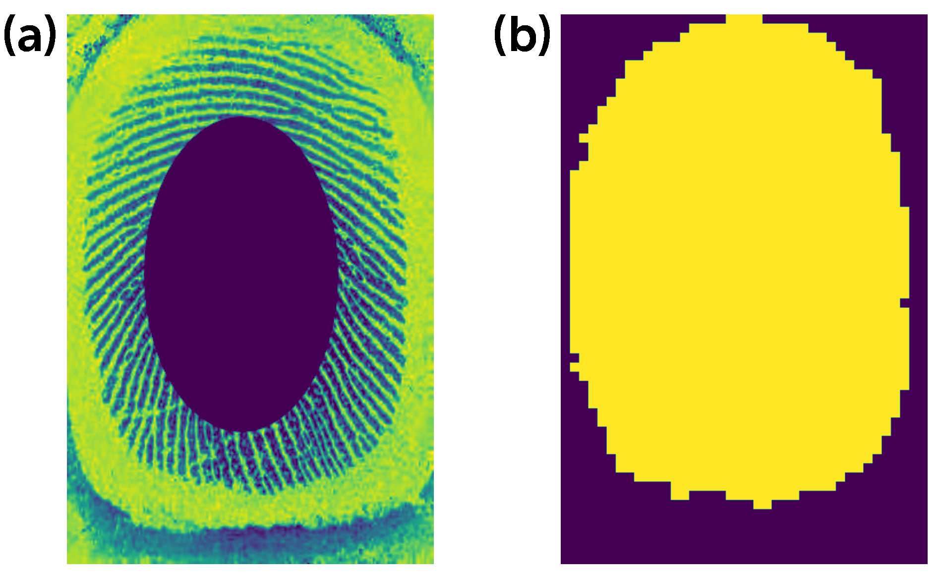
Figure 1: Input image (a) and a mask (b)

While preparing the cleanup data, we tried out different methods of image binarization (Fig. 2.a), where we tested different cutoff parameters and algorithms. However due to the types of input data, many did not provide acceptable results. The major problem was a merging papillary pattern. As a result, we decided to use an adaptive binarization algorithm that involves using the 'mean' metrics (Fig. 2.b), which, in our opinion, was the best option out of all the methods we have tested.

If you are interested, you can find the comparisons of image binarization methods by following this link.

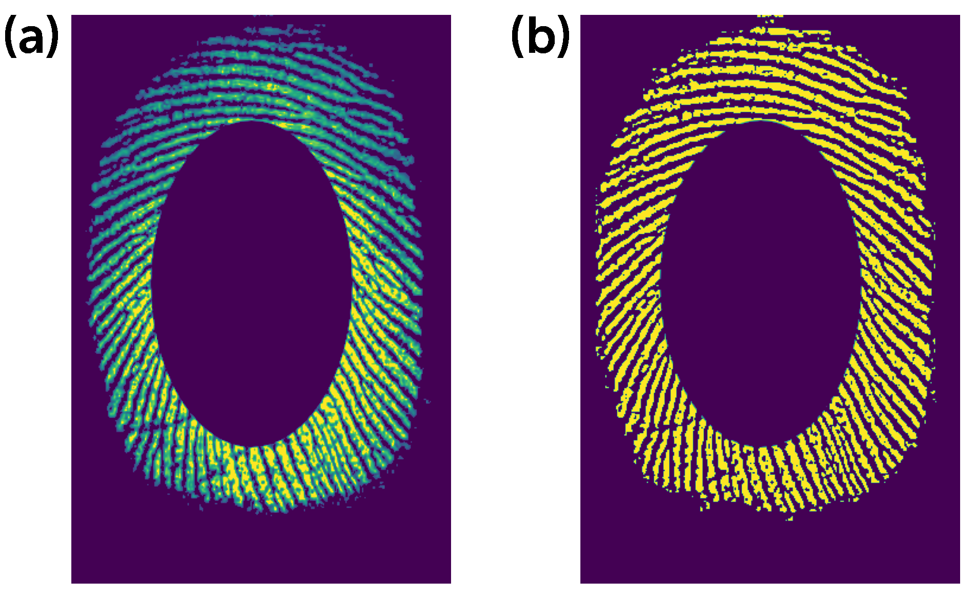
Figure 2: Normal (a) and adaptive binarization (b)

First option

Once we have sorted out the data, we moved on to the designing the neural network's structure. As our first option, we chose the auto-encoder (see Figure 3).

We implemented the so-called Binary Auto-encoder. You can read more about it here. We were therefore expecting the auto-encoder's latency layer (z layer in Figure 3) to act as the input fingerprint's hash, however, it turned out to be much trickier than expected and we shall tell you why later on.

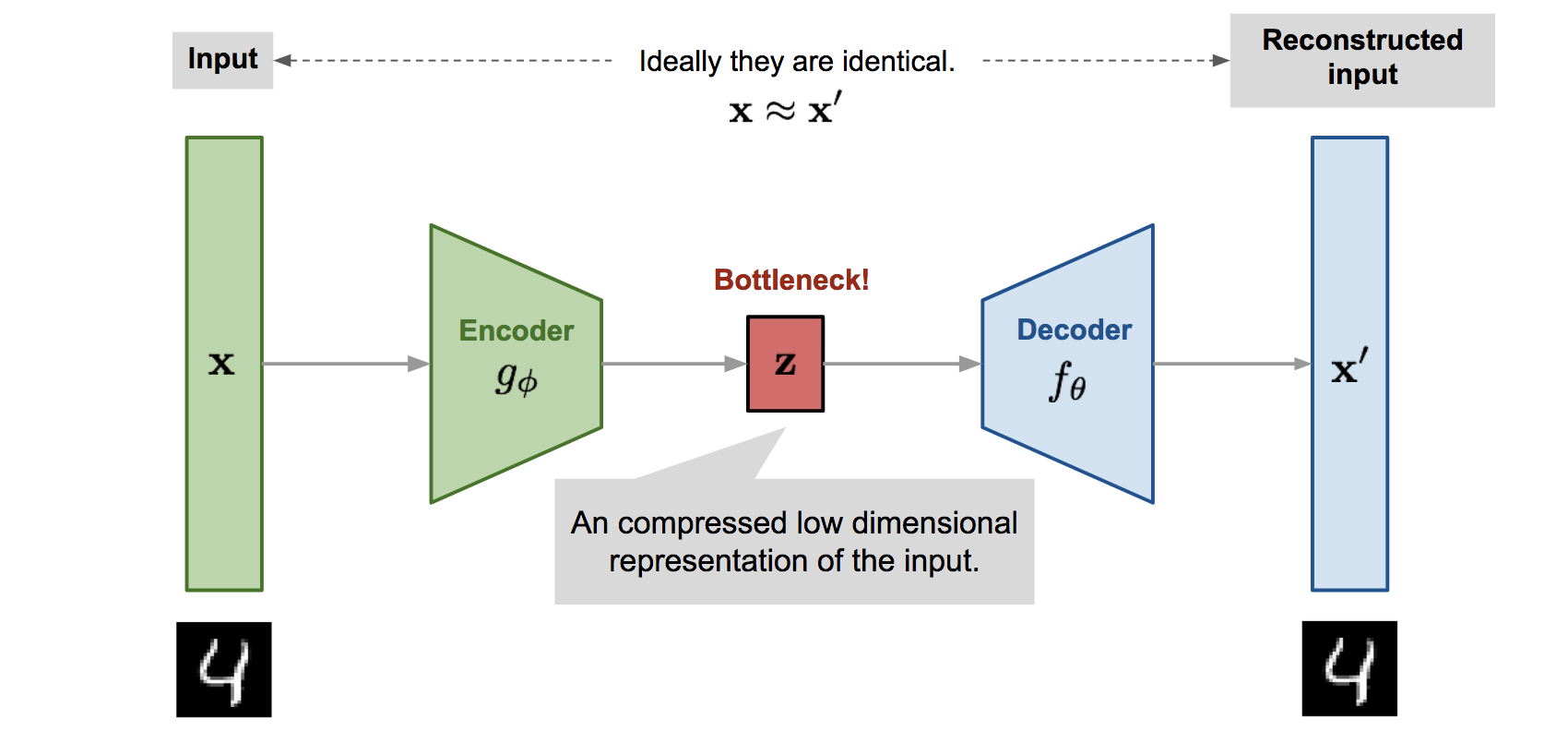
Figure 3: Auto-encoder's architecture.

Training the auto-encoder is quite a simple process, compared to other architectures. First, we take the data and divide it into two samples: data for training and data for validation. We usually divide it in the following proportion: 90% for training and 10% for validation. It's convenient to use the function from the scikit-learn library to divide it.

We use Adam's algorithm, as the optimizer, and BinaryCrossentropy as the loss function. Moving onto the encoder and decoder, we use the  Conv2D and MaxPooling2D, as pooling layers, as using only the Dense layer makes little sense due to a high number of links between layers in large input images.

Now it only remains to train it for 100-200 eras until we reach a plateau in the model's accuracy. Figure 4 shows the training graph of the auto-encoder, which we trained for 100 eras.

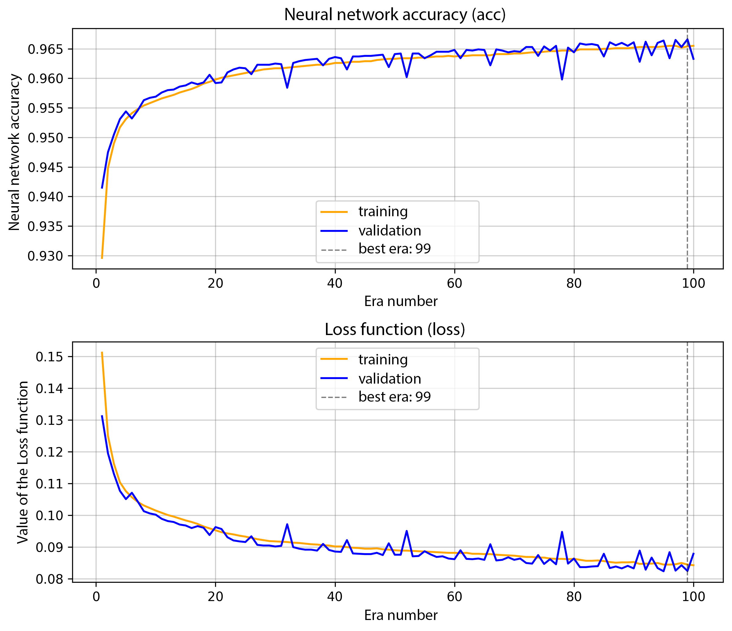
Figure 4: Auto-encoder learning graph.

The result of auto-encoder training was an accuracy rate of 96%. On the 5.b image you can see how the auto-encoder did an excellent job at restoring the original image.

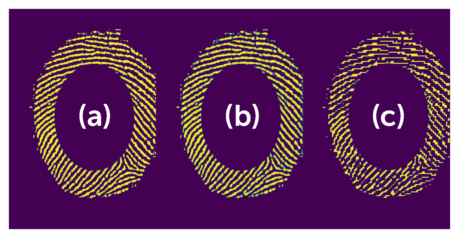
Figure 5: Input (a), restored (b) and rounded restored (c) image.

We used several metrics as a comparison measure for output vectors (read as the latency layer):

• Hamming's distance;
• Indel's distance;
• Levenstein'sdistance.

For this purpose, we used the sigmoid in the output layer of the encoder model as an activation layer. After that, the encoder’s output vector had to be binarized and we needed the result to be used for comparison.

However, this approach didn't lead to success, as it was not possible to separate the two classes of images. In Figure 6, you can see that it is impossible to distinguish the cutoff border, when the fingerprints can be classified as 'matched'. The X-axis represents the Hamming's distance, whereas the Y-axis is chosen as a class - 1 = matches and 0 = doesn't match.

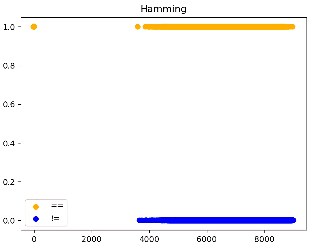
Figure 6: Calculation of the Hamming distance for fingerprints. Yellow - fingerprints match, blue - fingerprints do not match.

After comparing the two, we examined what the latency layer was and found out that the auto-encoder was reducing the input image size instead of extracting features from the fingerprint data.

At this point we decided to stop experimenting with the auto-encoder and search for another architecture for our task.

Sudden insight

After several long attempts to get something meaningful out of the auto-encoder, we constructed the simplest architecture possible. It turns out that the simplest solution to this problem ended up being the best one.

The first model (coder) will encode the input image into some intermediate state. To be precise, it is simply a set of several convolutions that reduce the input image to a 30x20 vector.

The second model (predictor) will compare the convolution vectors and conclude whether the two fingerprints are similar or not.

The resulting model (base) simply combines both. We did this to make the training process more convenient. Also, we constructed the models to enable them being used individually.

Figure 7 schematically demonstrates the neural network's architecture.

Figure 7: Schematic representation of the neural network's architecture.

Results

As a result of neural network's operation, you can get a resulting vector after the coder's model. Then it can be used for comparison with another vector (via the predictor model) or placed in a database. An example of such a vector is in Figure 8.

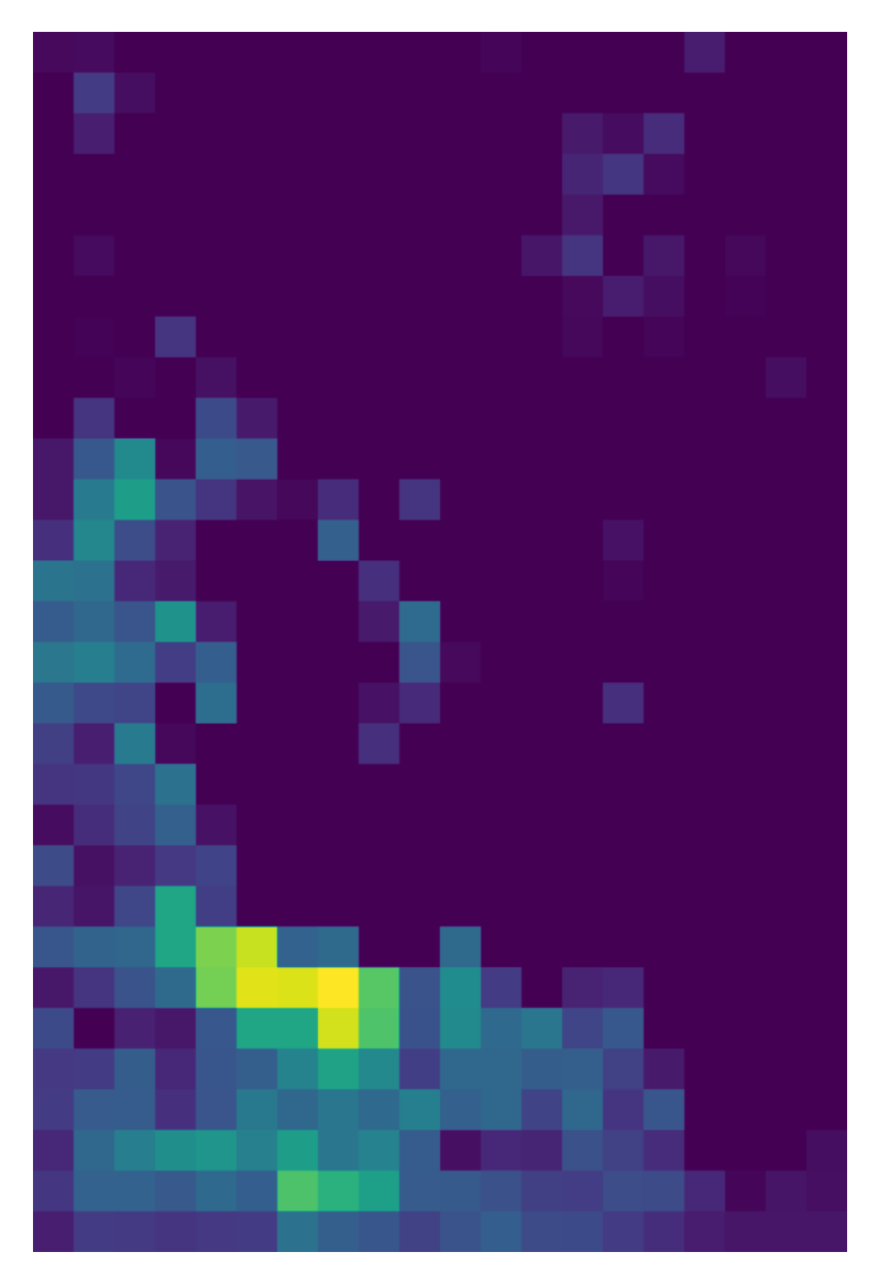
Figure 8: An output vector (30x20) after the coder's model (image has been zoomed in)

During the course of training, we achieved the following results, as presented in the Table , and in Figure 9. The test was carried out on a selection of 20,000 elements, with one half representing the "fingerprints match" class and the other half representing the "fingerprints do not match" class.

Table 1: Metrics for assessing the accuracy of the trained model.

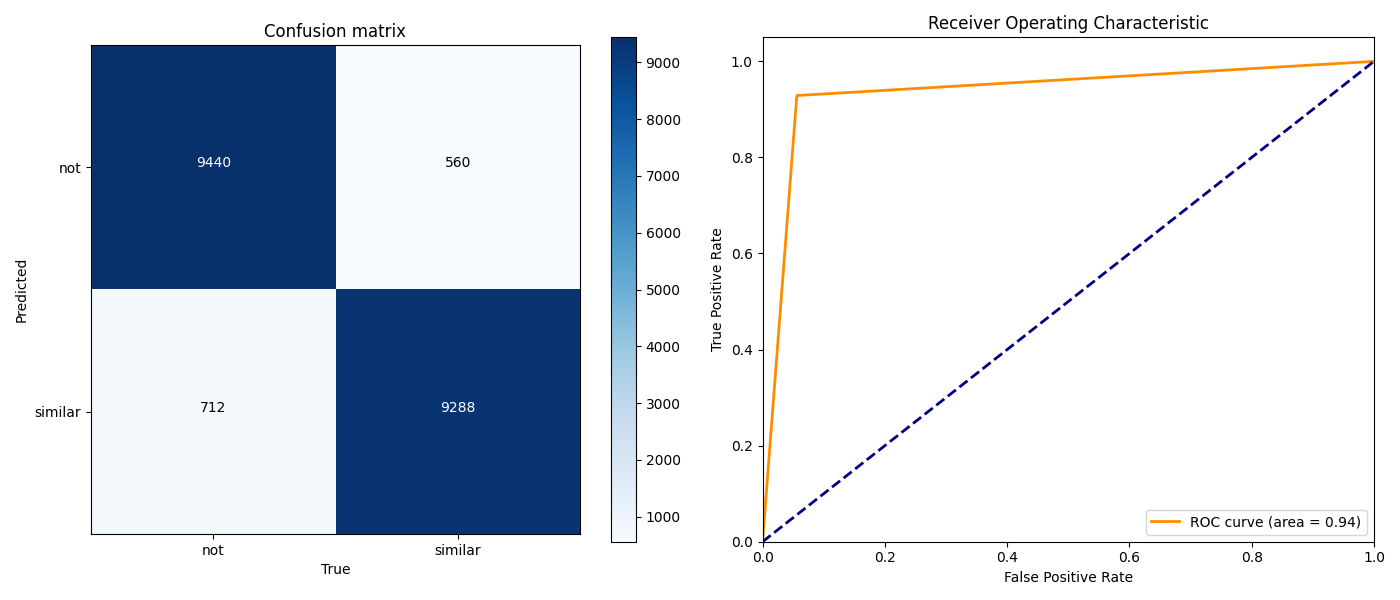
Figure 9: Error matrix and the ROC curve.

Conclusion

Developing neural networks is always an interesting and diverse process, and this project is not an exception. Working with biometrics is always a challenge for the team, and our machine learning engineers not only applied the accumulated knowledge, but also expanded their expertise with the approaches that have been tested throughout the project. Just as before, the MST company is ready to solve the most non-standard tasks and offer its clients the highest quality of neural network and software products development.